Workshop: Machine Learning - Part 1 - Classification
15 May 2021, Carlos Pena
This post is a conversion from an old workshop of mine. For a better view, please check the notebook.
Part One - Theory
#General Purpose
import numpy as np
import pandas as pd
import matplotlib.pyplot as plt
import seaborn as sns

#Data transform
from sklearn.utils import resample
from sklearn.model_selection import train_test_split
from sklearn.preprocessing import OneHotEncoder
from sklearn.preprocessing import LabelEncoder
from sklearn.preprocessing import MinMaxScaler
from sklearn.preprocessing import Normalizer
from sklearn.manifold import TSNE

#Model
from sklearn.neighbors import KNeighborsClassifier
from sklearn.tree import DecisionTreeClassifier
from sklearn.tree import export_text

#Metrics
from sklearn.metrics import accuracy_score, classification_report
from sklearn.metrics import f1_score, confusion_matrix, matthews_corrcoef

# Sample Datasets
from sklearn.datasets import load_iris

sns.set_theme()
Dataset
iris         = load_iris()
iris_data    = iris.data
iris_target  = iris.target
iris_targ_n  = iris['target_names']
iris_targ_n  = iris_targ_n[iris.target]
iris_feat_n  = iris['feature_names']

df = pd.DataFrame(iris_data, columns=iris_feat_n)
df['target'] = iris_targ_n
df.head()
| sepal length (cm) | sepal width (cm) | petal length (cm) | petal width (cm) | target | |
|---|---|---|---|---|---|
| 0 | 5.1 | 3.5 | 1.4 | 0.2 | setosa |
| 1 | 4.9 | 3.0 | 1.4 | 0.2 | setosa |
| 2 | 4.7 | 3.2 | 1.3 | 0.2 | setosa |
| 3 | 4.6 | 3.1 | 1.5 | 0.2 | setosa |
| 4 | 5.0 | 3.6 | 1.4 | 0.2 | setosa |
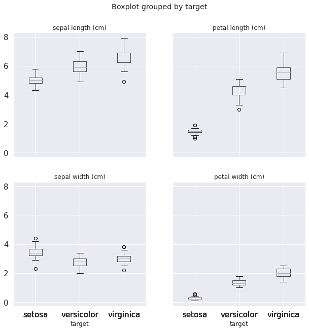
axes = df.boxplot(column=[iris_feat_n[0], iris_feat_n[2], iris_feat_n[1], iris_feat_n[3]],
                  by='target', figsize=(10, 10), fontsize=15)
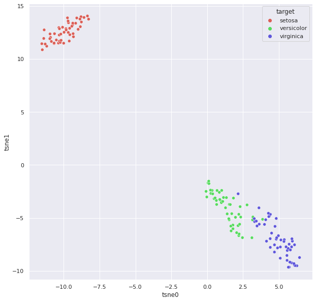
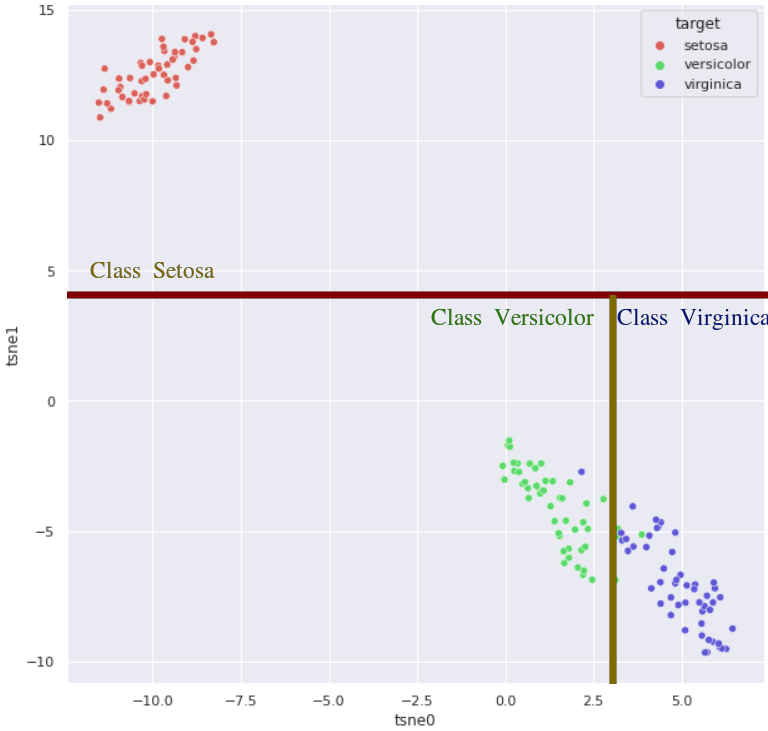
np.random.seed(2021)

tsne = TSNE(n_components=2, verbose=0, perplexity=40, n_iter=300)
tsne_results = tsne.fit_transform(iris_data)

df['tsne0'] = tsne_results[:, 0]
df['tsne1'] = tsne_results[:, 1]

plt.figure(figsize=(10,10))
sns.scatterplot( x="tsne0", y="tsne1", hue="target",
    palette=sns.color_palette("hls", 3), data=df,
    legend="full", alpha=1);
Models
“A computer program is said to learn from experience E with respect to some class of tasks T and performance measure P, if its performance at tasks in T, as measured by P, improves with experience E.” - Tom Mitchell
Dado uma tarefa T medida por uma métrica P, se a métrica P melhorar com a experiência E é dito que o modelo aprendeu.
Dado a tarefa (classificação entre gato-cachorro) e uma métrica (taxa de acerto), se a métrica (taxa de acerto) melhorar com a experiência (fotos de gatos-cachorros) é dito que o modelo aprendeu.
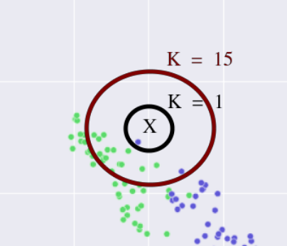
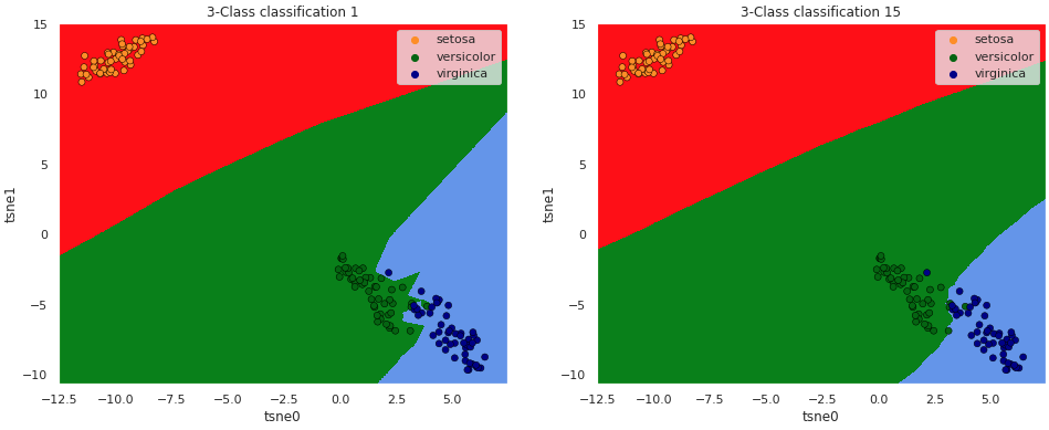
K-Nearest Neighbors
Árvore de decisão (Decision tree)
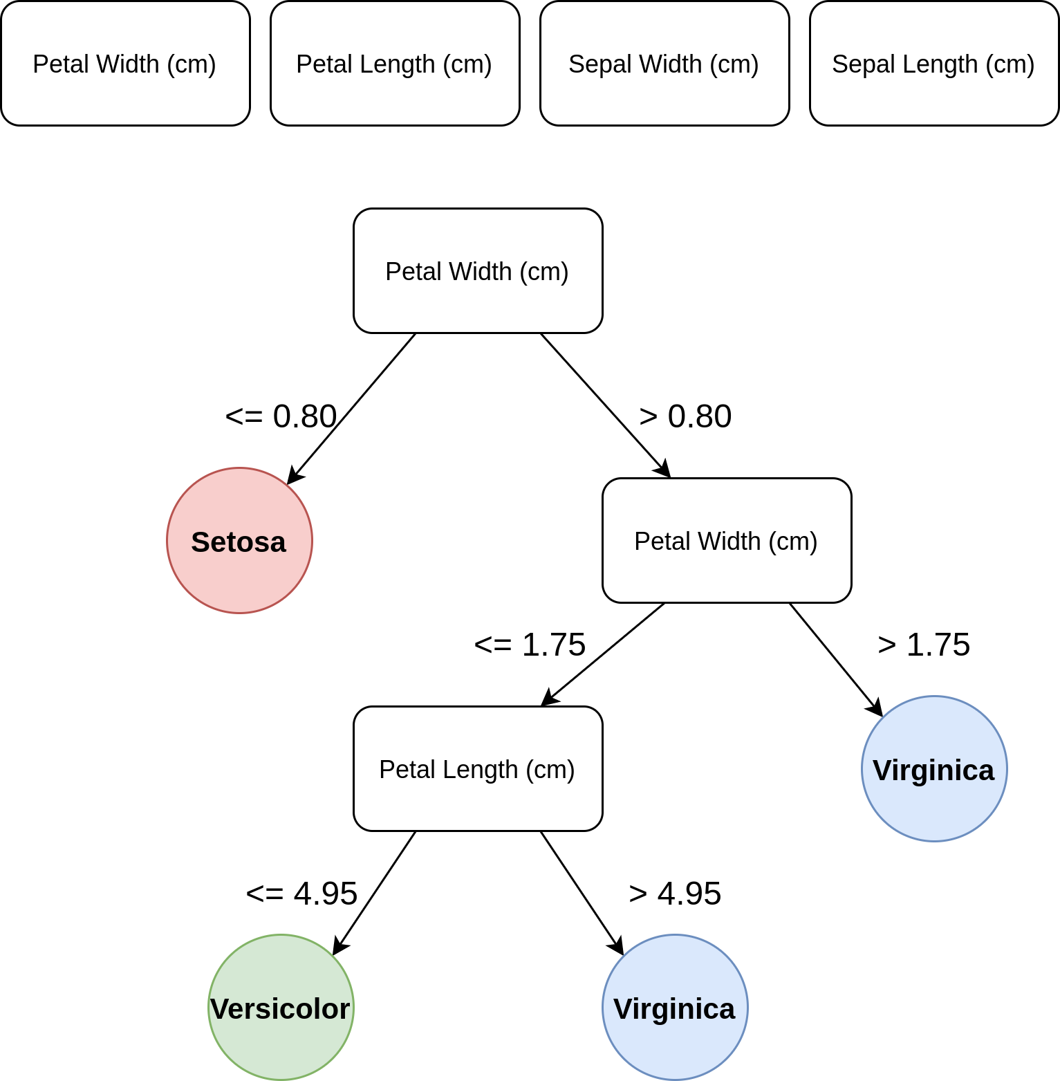
decision_tree = DecisionTreeClassifier(random_state=2021, max_depth=3)
decision_tree = decision_tree.fit(iris_data, iris_target)
r = export_text(decision_tree, feature_names=iris['feature_names'])
Metrics
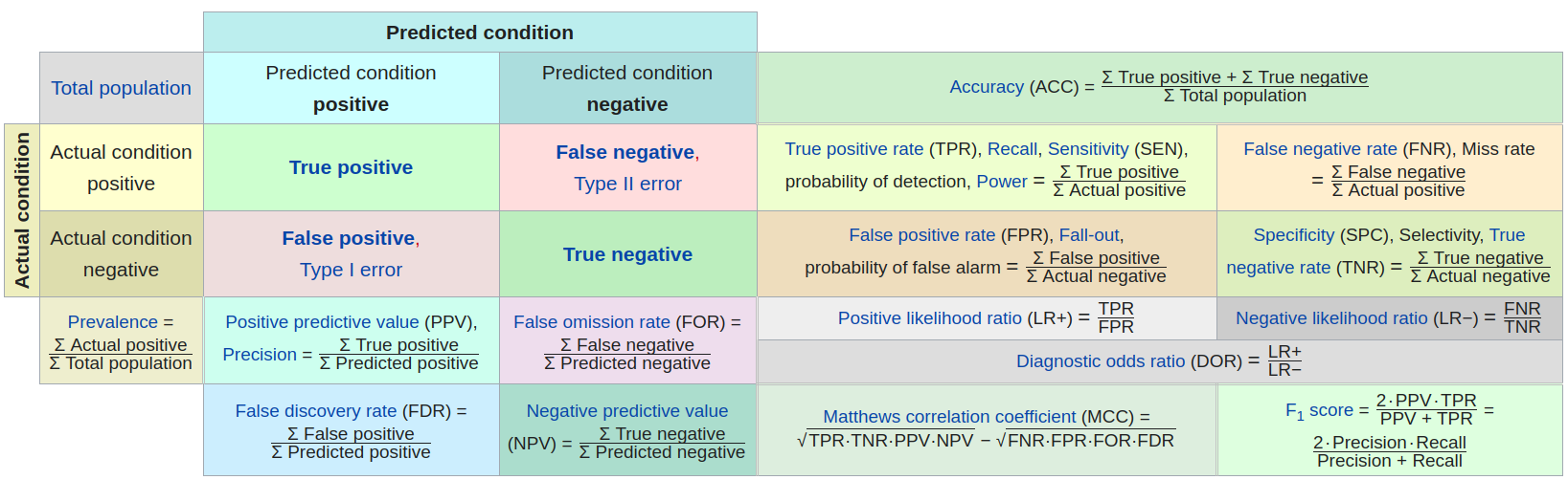 Source: https://en.wikipedia.org/wiki/Confusion_matrix
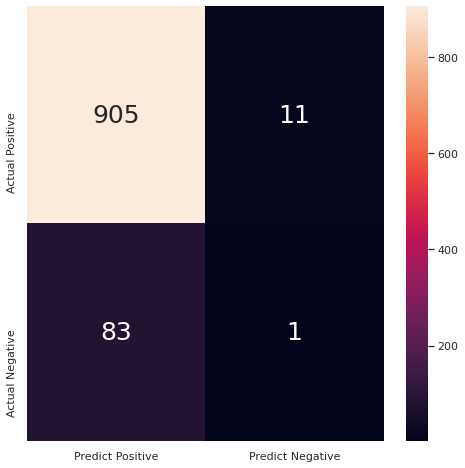
np.random.seed(2021)
has_cancer = (np.random.random(size=1000) > 0.9).astype(int)
predicted  = (np.random.random(size=1000) > 0.99).astype(int)#np.zeros(shape=1000, dtype=int)

cm = confusion_matrix(has_cancer, predicted)

df_cm = pd.DataFrame(cm, index = ["Actual Positive", "Actual Negative"],
                      columns = ["Predict Positive", "Predict Negative"])
plt.figure(figsize = (8,8))
axes = sns.heatmap(df_cm, annot=True, fmt='g', annot_kws={"size": 25})
plt.show()

accuracy = accuracy_score(has_cancer, predicted)
f1       = f1_score(has_cancer, predicted)
mcc      = matthews_corrcoef(has_cancer, predicted)
print(f"Results: Accuracy {accuracy:0.3f}\n         F1       {f1:0.3f}",
      f"\n         MCC     { mcc:0.3f}")

    Results: Accuracy 0.906
             F1       0.021
             MCC     -0.000
Part Two - Practice
UCI Machine Learning Repository: Iris
Kaggle: Titanic Machine Learning from Disaster – Extra
data = pd.read_csv('../data/kaggle-titanic-train.csv')
data.head(10)
| PassengerId | Survived | Pclass | Name | Sex | Age | SibSp | Parch | Ticket | Fare | Cabin | Embarked | |
|---|---|---|---|---|---|---|---|---|---|---|---|---|
| 0 | 1 | 0 | 3 | Braund, Mr. Owen Harris | male | 22.0 | 1 | 0 | A/5 21171 | 7.2500 | NaN | S |
| 1 | 2 | 1 | 1 | Cumings, Mrs. John Bradley (Florence Briggs Th... | female | 38.0 | 1 | 0 | PC 17599 | 71.2833 | C85 | C |
| 2 | 3 | 1 | 3 | Heikkinen, Miss. Laina | female | 26.0 | 0 | 0 | STON/O2. 3101282 | 7.9250 | NaN | S |
| 3 | 4 | 1 | 1 | Futrelle, Mrs. Jacques Heath (Lily May Peel) | female | 35.0 | 1 | 0 | 113803 | 53.1000 | C123 | S |
| 4 | 5 | 0 | 3 | Allen, Mr. William Henry | male | 35.0 | 0 | 0 | 373450 | 8.0500 | NaN | S |
| 5 | 6 | 0 | 3 | Moran, Mr. James | male | NaN | 0 | 0 | 330877 | 8.4583 | NaN | Q |
| 6 | 7 | 0 | 1 | McCarthy, Mr. Timothy J | male | 54.0 | 0 | 0 | 17463 | 51.8625 | E46 | S |
| 7 | 8 | 0 | 3 | Palsson, Master. Gosta Leonard | male | 2.0 | 3 | 1 | 349909 | 21.0750 | NaN | S |
| 8 | 9 | 1 | 3 | Johnson, Mrs. Oscar W (Elisabeth Vilhelmina Berg) | female | 27.0 | 0 | 2 | 347742 | 11.1333 | NaN | S |
| 9 | 10 | 1 | 2 | Nasser, Mrs. Nicholas (Adele Achem) | female | 14.0 | 1 | 0 | 237736 | 30.0708 | NaN | C |
data_filter_col = data[['Pclass', 'Sex', 'Age', 'SibSp', 'Parch', 'Fare', 'Survived']]
data_filter_col.head()
| Pclass | Sex | Age | SibSp | Parch | Fare | Survived | |
|---|---|---|---|---|---|---|---|
| 0 | 3 | male | 22.0 | 1 | 0 | 7.2500 | 0 |
| 1 | 1 | female | 38.0 | 1 | 0 | 71.2833 | 1 |
| 2 | 3 | female | 26.0 | 0 | 0 | 7.9250 | 1 |
| 3 | 1 | female | 35.0 | 1 | 0 | 53.1000 | 1 |
| 4 | 3 | male | 35.0 | 0 | 0 | 8.0500 | 0 |
data_filter_col['Sex'].replace(['female','male'],[1,0],inplace=True)
data_filter_col.isnull().sum()

    Pclass        0
    Sex           0
    Age         177
    SibSp         0
    Parch         0
    Fare          0
    Survived      0
    dtype: int64
data_filter_col = data_filter_col.dropna()

data_filter_col.shape
(714, 7)
X = data_filter_col[['Pclass', 'Sex', 'Age', 'SibSp', 'Parch', 'Fare']]
y = data_filter_col['Survived']

X.head(2)
| Pclass | Sex | Age | SibSp | Parch | Fare | |
|---|---|---|---|---|---|---|
| 0 | 3 | 0 | 22.0 | 1 | 0 | 7.2500 |
| 1 | 1 | 1 | 38.0 | 1 | 0 | 71.2833 |
corr = data_filter_col.corr()
corr.style.background_gradient(cmap='coolwarm')
| Pclass | Sex | Age | SibSp | Parch | Fare | Survived | |
|---|---|---|---|---|---|---|---|
| Pclass | 1.000000 | -0.155460 | -0.369226 | 0.067247 | 0.025683 | -0.554182 | -0.359653 |
| Sex | -0.155460 | 1.000000 | -0.093254 | 0.103950 | 0.246972 | 0.184994 | 0.538826 |
| Age | -0.369226 | -0.093254 | 1.000000 | -0.308247 | -0.189119 | 0.096067 | -0.077221 |
| SibSp | 0.067247 | 0.103950 | -0.308247 | 1.000000 | 0.383820 | 0.138329 | -0.017358 |
| Parch | 0.025683 | 0.246972 | -0.189119 | 0.383820 | 1.000000 | 0.205119 | 0.093317 |
| Fare | -0.554182 | 0.184994 | 0.096067 | 0.138329 | 0.205119 | 1.000000 | 0.268189 |
| Survived | -0.359653 | 0.538826 | -0.077221 | -0.017358 | 0.093317 | 0.268189 | 1.000000 |
X.describe()
| Pclass | Sex | Age | SibSp | Parch | Fare | |
|---|---|---|---|---|---|---|
| count | 714.000000 | 714.000000 | 714.000000 | 714.000000 | 714.000000 | 714.000000 |
| mean | 2.236695 | 0.365546 | 29.699118 | 0.512605 | 0.431373 | 34.694514 |
| std | 0.838250 | 0.481921 | 14.526497 | 0.929783 | 0.853289 | 52.918930 |
| min | 1.000000 | 0.000000 | 0.420000 | 0.000000 | 0.000000 | 0.000000 |
| 25% | 1.000000 | 0.000000 | 20.125000 | 0.000000 | 0.000000 | 8.050000 |
| 50% | 2.000000 | 0.000000 | 28.000000 | 0.000000 | 0.000000 | 15.741700 |
| 75% | 3.000000 | 1.000000 | 38.000000 | 1.000000 | 1.000000 | 33.375000 |
| max | 3.000000 | 1.000000 | 80.000000 | 5.000000 | 6.000000 | 512.329200 |
X_train, X_val, y_train, y_val = train_test_split(
                    X, y, test_size=0.30, random_state=2021)
tree = DecisionTreeClassifier()

tree.fit(X_train, y_train)

predicted_val = tree.predict(X_val)
predicted_train = tree.predict(X_train)

acc_train = accuracy_score(y_train, predicted_train)
acc_val = accuracy_score(y_val, predicted_val)
print(f"Accuracy: Train {acc_train:0.3f} | Val {acc_val:0.3f}")

report = classification_report(y_val, predicted_val)
print(report)

    Accuracy: Train 0.990 | Val 0.744

                  precision    recall  f1-score   support

               0       0.78      0.79      0.78       126
               1       0.69      0.69      0.69        89

        accuracy                           0.74       215
       macro avg       0.74      0.74      0.74       215
    weighted avg       0.74      0.74      0.74       215
knn = KNeighborsClassifier(n_neighbors=5)

knn.fit(X_train, y_train)

predicted_val = knn.predict(X_val)
predicted_train = knn.predict(X_train)

acc_train = accuracy_score(y_train, predicted_train)
acc_val = accuracy_score(y_val, predicted_val)
print(f"Accuracy: Train {acc_train:0.3f} | Val {acc_val:0.3f}")

report = classification_report(y_val, predicted_val)
print(report)

    Accuracy: Train 0.796 | Val 0.656
                  precision    recall  f1-score   support

               0       0.69      0.75      0.72       126
               1       0.59      0.53      0.56        89

        accuracy                           0.66       215
       macro avg       0.64      0.64      0.64       215
    weighted avg       0.65      0.66      0.65       215
norm = Normalizer()
X_train = norm.fit_transform(X_train)
X_val   = norm.transform(X_val)

knn = KNeighborsClassifier(n_neighbors=5)
knn.fit(X_train, y_train)

predicted_val = knn.predict(X_val)
predicted_train = knn.predict(X_train)

acc_train = accuracy_score(y_train, predicted_train)
acc_val = accuracy_score(y_val, predicted_val)
print(f"Accuracy: Train {acc_train:0.3f} | Val {acc_val:0.3f}")

report = classification_report(y_val, predicted_val)
print(report)

    Accuracy: Train 0.820 | Val 0.721
                  precision    recall  f1-score   support

               0       0.74      0.82      0.77       126
               1       0.69      0.58      0.63        89

        accuracy                           0.72       215
       macro avg       0.71      0.70      0.70       215
    weighted avg       0.72      0.72      0.72       215